In the world of data and computer programs, the concept of Machine Learning might sound like a tough nut to crack, full of tricky math and complex ideas.
This is why today I want to slow down and check out the basic stuff that makes all this work with a new issue of my MLBasics series.
Today’s agenda is to understand Support Vector Machines.
This powerful tool helps us classify data into distinct categories, but…
how does it work?
Let’s try to simplify the Support Vector Machines model👇🏻
What is a Support Vector Machine?
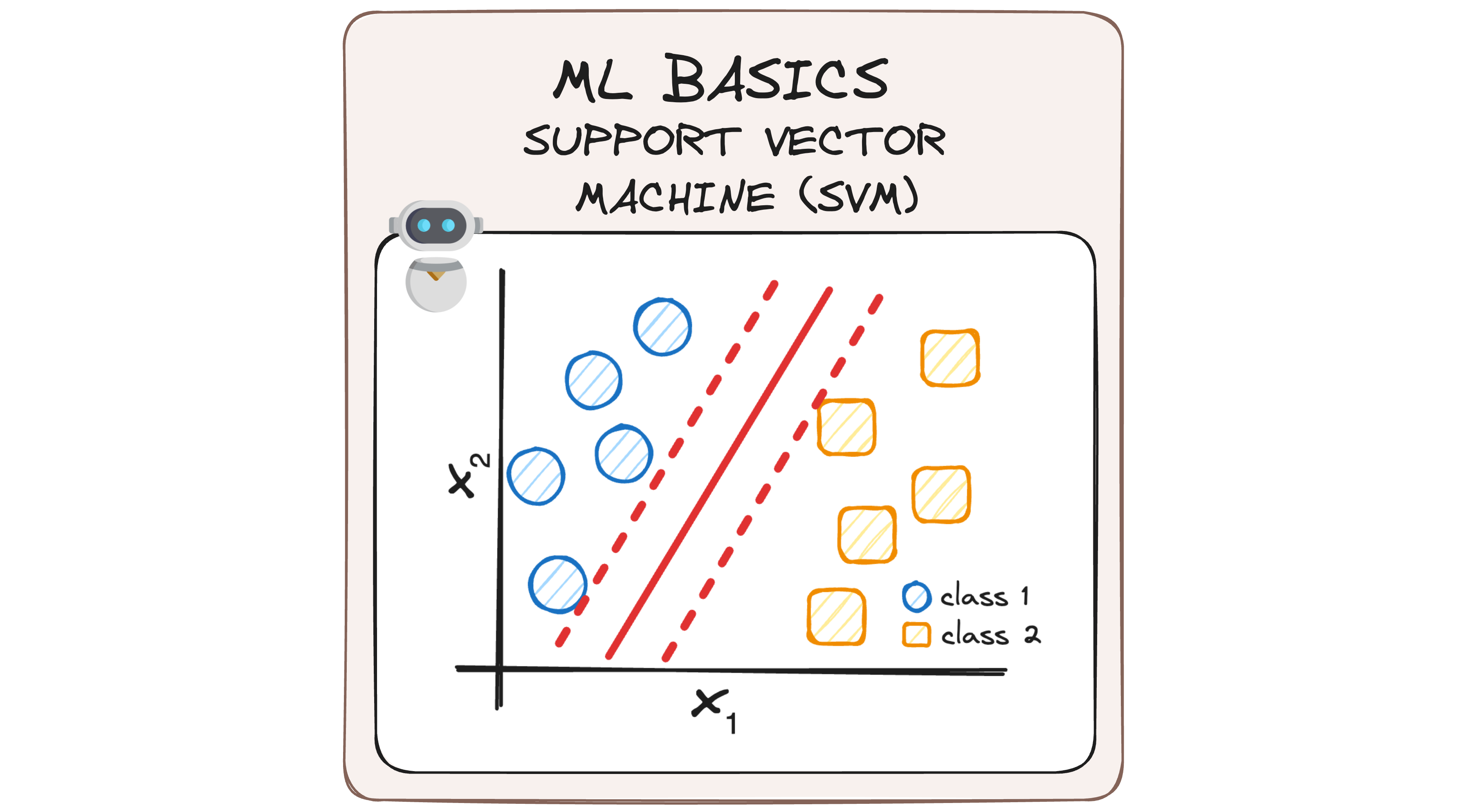
A Support Vector Machine (SVM) is a supervised ML algorithm that aims to find a hyperplane that best separates data points into two different classes.
The challenge is that there are infinitely many possible hyperplanes that can do this. So, the goal of SVM is to identify the hyperplane that best separates the classes with the maximum margin.

Key Concepts in SVM
Before we delve deeper, let’s understand some key terms:
- Support Vectors: These are the data points closest to the hyperplane and highly influence its position and orientation.
- Margin: The margin is the distance between the hyperplane and the nearest data point from either class. A larger margin implies a better generalization of the classifier.
- Hyperplane: In a two-dimensional space, this is a line that separates the data into two parts. In higher dimensions, it’s a plane or a higher-dimensional analog.

How Does SVM Work?
Imagine you have a dataset with two types of data points:
- Blue 🔵
- Yellow 🟨
You want to classify new data points as either blue or yellow. The main challenge is that numerous possible hyperplanes can separate the two classes, so there’s a big question:
How to find the best hyperplane?

The best hyperplane is the one that has the maximum distance from both classes. This is done by finding different possible hyperplanes and selecting the one with the maximum distance from both classes.
Mathematical Intuition Behind SVM
To understand how SVM classifies data, let’s dive into some mathematics.
The dot product is the projection of one vector along with another. So we can take advantage of it to determine whether a point is on one side of the hyperplane or the other.
If we consider a random point X:
- If X⋅W > c – It’s a positive sample.
- If X⋅W < c – It’s a negative sample.
- If X⋅W = c – It’s on the decision boundary.
Easy, right?

So let’s rewind a bit and understand where these equations come from:
1. Determining how to find the hyperplane
To achieve our "splitting line", we can first calculate the distance d between the support vectors and the hyperplane. The margin is twice the distance from the hyperplane to the nearest support vector, as no points should lie within this margin.
2. Projecting the Distance "d"
The distance d can be obtained by projecting the difference between two support vectors onto the direction of the normal vector w of the hyperplane.

I’m pretty sure many of you have no idea how we got here, so let’s step back and understand better what this function means from the beginning.
Let’s imagine we have two vectors: A and B, that generate a θ degree between them. We can easily find the projection of A over B using the scalar product.
This means that we can find the projection of A over B knowing both A and B vectors, as you can observe in the following formulas.

So now that we understand these basics, let’s go back to our SVM model. We can apply the same mathematical concept to SVM, considering that A is the vector defined by both support vector machines and B is the normal vector of our splitting hyperplane.

3. Defining the Constraints
Now we can define the constraints using our margins. We know that the Maximum Margin Hyperplane must follow a line equation (in our 2D example).

This means that anything that lies upon it will have a positive value (corresponding to the positive hyperplane) and anything below this will have a negative value (corresponding to the negative hyperplane).
The separation between these two hyperplanes is what we know as "margin".
Margin in SVM
The margin is a critical concept in SVM, serving as a buffer zone around the hyperplane where no data points are present. The wider this margin, the better the model can generalize to unseen data, reducing the likelihood of overfitting.
To classify points as positive or negative, we establish a decision rule based on their position relative to the hyperplane.
- Points on one side are classified into one category (blue 🔵 )
- Points on the other side fall into the opposite category (yellow 🟨).
By maximizing the margin, SVM ensures that the decision boundary is optimally positioned to separate the classes with the highest possible confidence.
So how do we maximize it?
Optimization and Constraints
SVM involves solving an optimization problem to maximize the margin. This involves ensuring that the chosen hyperplane maintains a sufficient distance from the nearest data points of each class, referred to as support vectors.
We already have our classification algorithm based on the line equations we found before. So we can define that the output will be:
- +1 or 🔵 for the data lying in the positive side.
- -1 or 🟨 for the data lying in the negative side.

But we still need to find both the w vector and the b parameter.
So… what can we do?
We know that the support vectors, which lie on the margin boundaries, fulfill the following constraints, as they are contained within our positive and negative hyperplanes.

So we can easily generalize this into a…
General Constraint Equation
To ensure that no positive or negative data points cross the margin, the constraints for all data points (x,y) can be summarized as:

And there’s only one more step to be performed…
Optimization Objective
Now that we have our general constraint equation, we can minimize the absolute of the vector w while satisfying the constraints.
This can be mathematically formulated as:

By solving this optimization problem, we find the optimal values of the vector w and b that define the hyperplane with the maximum margin, ensuring the best possible separation between the classes.
Conclusion
Support Vector Machines are a powerful tool in the arsenal of a data scientist offering an effective method for binary classification.
By focusing on maximizing the margin between classes, SVMs create robust classifiers that generalize well to new data, reducing the risk of overfitting.
The mathematical foundation of SVMs ensures the identification of the optimal hyperplane, making them a reliable choice for various classification tasks.
Whether you’re dealing with complex datasets or looking to improve your model’s performance, understanding and implementing SVMs can significantly enhance your machine-learning toolkit.
Did you like this MLBasics issue? Then you can subscribe to my DataBites Newsletter to stay tuned and receive my content right to your mail!
I promise it will be unique!

Check out these great Data Science roadmaps to become a Data Scientist or Data Engineer among others! 🤓
You can also find me on X, Threads, and LinkedIn, where I post daily cheatsheets about ML, SQL, Python, and DataViz.
Some other nice articles you should go check out! 😀
Breaking down Logistic Regression to its basics
MLBasics – Simple Linear Regression
Simplifying Multiple Linear Regression – A Beginner’s Guide with Height, Weight, and Sex


