Linear Regression, Logistic Regression, and SVM in 10 Minutes

Machine Learning

Table of contents

· So, how does machine learning work?
· Linear Models
  ∘ Linear regression
  ∘ Ridge
  ∘ Lasso
  ∘ Elastic-Net
· Logistic Regression
· Support Vector Machine (SVM)
  ∘ Classification
  ∘ Regression
  ∘ Kernel functions
· A note on preprocessing
· Conclusion

Machine learning modeling is a data scientist’s problem solver. Even though it doesn’t take the majority of our time, it’s personally much more fun than data cleaning.

To be frank, some models are mathematically involved. The good news is, as a data scientist, you aren’t necessarily capable to build machine learning models from scratch. There is already a plethora of libraries to choose a model from and there’s no need to reinvent the wheel. However, it’s always good to know how a model works from a bird’s-eye view.

So, how does machine learning work?

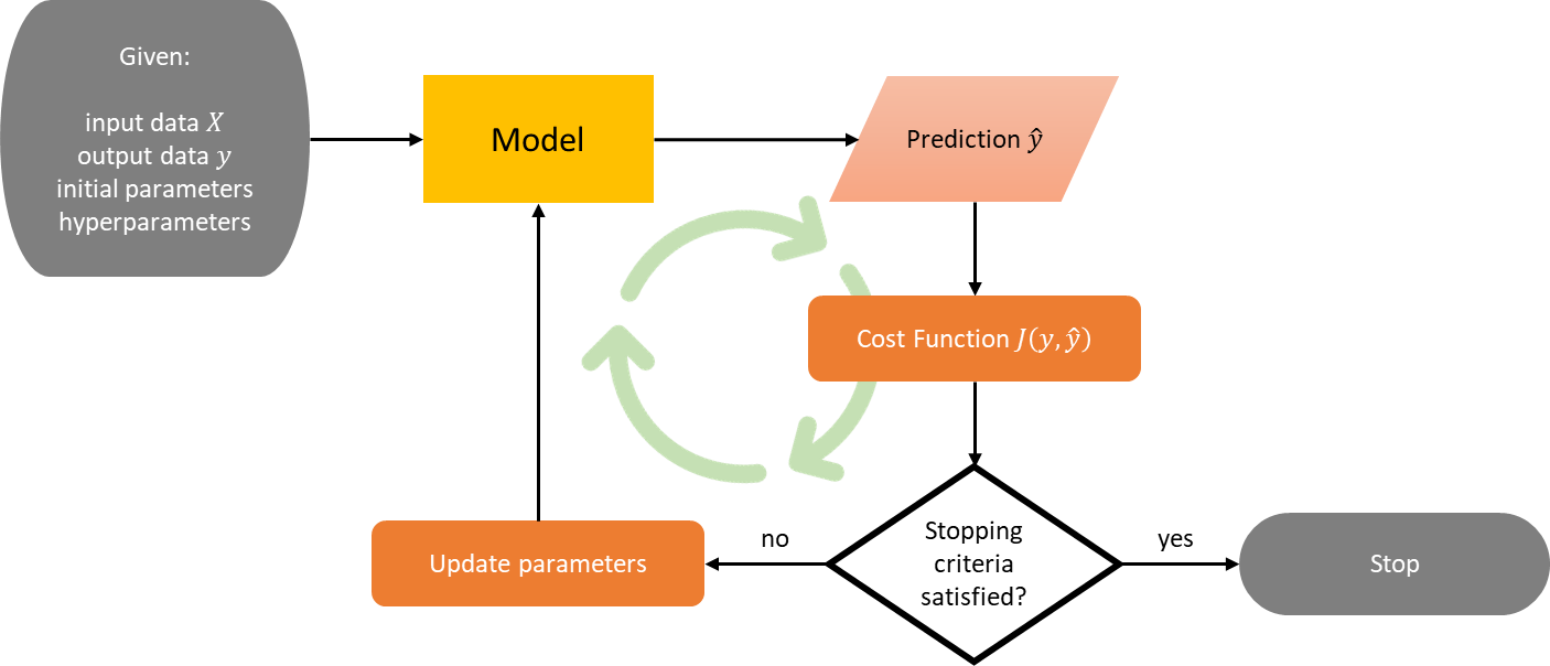
In general, all supervised machine learning models work in the same way: you have input data X and output data y, then the model finds a map from X to y. That’s why machine learning is called that way: instead of us deliberately coding the logic that maps X to y, the model learns on its own by updating its parameters. Most models also have hyperparameters, i.e. parameters that can’t be learned and need to be tuned by the user.

To be clear, let’s say you have m observations and n features, and you’re working on a single-output task. Then, X is an m × n matrix and y is a vector of size m. To learn the mapping from X to y, the model will have to find the optimum parameters using an optimizer, such as gradient descent, BFGS, and many more. But what does it mean to be optimum? Optimum in terms of what, exactly?

You can see the "find optimum parameters" problem as an optimization problem (yes, machine learning really is just an optimization problem). So, you need an objective function, or in other literature is also called a cost function.

Cost functions are different depending on the model and task. For example, for linear regression with predicted parameter w, a familiar cost function would be the sum of squared error, denoted by

Optimum w is found when w minimizes this cost function.

Linear Models

In linear models and logistic regression below, we omit the bias coefficient b for convenience. The bias coefficient allows our models to be more general and there are two ways to add it:

1. By creating a column of ones in X so X is now an m × (n+1) matrix and w is a vector of size n+1, the notation Xw stays like that.
2. By explicitly changing Xw into Xw + b.

Linear regression

In linear regression, the target value ŷ is expected to be a linear combination of the features. In other words,

As mentioned before, with this model you would minimize the sum of squared error with respect to w, that is,

Despite its simple form, linear regression has a problem. If some features in X are correlated, then (XᵀX)⁻¹ will be close to singular and w becomes highly sensitive to errors, resulting in overfitting. Luckily, there is a workaround: by giving a penalty to w if it’s too big.

This gives birth to the ridge, lasso, and elastic-net regression.

Ridge

To give a penalty to w, we need to add a quantity in terms of w to the cost function such that minimizing the cost function also minimizes this quantity. The quantity in question is the square of the Euclidean norm (also called L2-norm) of w multiplied by a hyperparameter α ≥ 0. The objective becomes

With this objective, the model is discouraged to be too complex and tends to shrink w toward zero. The larger the value of α, the greater the amount of shrinkage, and thus w becomes more robust to collinearity.

Lasso

There’s an alternative to ridge regression. Instead of shrinking all coefficients in w toward zero, your model can also learn to set some coefficients to zero. You’re left with a few non-zero coefficients, effectively reducing the number of dependent features.

The objective becomes surprisingly easy. We simply switch the square of the L2-norm in the cost function of ridge regression with the L1-norm as follows

With this capability, lasso regression is also useful for feature selection and reducing the dimensionality of X by selecting non-zero coefficients. The reduced data can then be used with another classifier/regressor. It’s easy to see that the higher the value of α, the fewer features selected.

Elastic-Net

It’s also possible to gain the advantage of both ridge and lasso regression. Elastic-net has both L1 and L2-norm in the cost function, allowing for learning a sparse model where few of the coefficients are non-zero like lasso, while still maintaining the regularization properties of rigde. The objective is now

The hyperparameter 0 ≤ ρ ≤ 1 is called L1-ratio which controls the combination of L1 and L2-norm. Note that if ρ = 0, then the objective is equivalent to ridge’s. On the other hand, if ρ = 1, then the objective is equivalent to lasso’s.

Below is an example of the application of linear models on the same data, where X has 4 features and bias b = 0. We can see that ridge shrinks the coefficients toward zero, lasso sets the first coefficient to zero, and elastic-net is like the combination of both.

Linear Regression
w = [ 2.7794 -11.3707  46.0162  32.4487]

Ridge
w = [ 2.2607  -9.8212  45.3181  31.9229]

Lasso
w = [-0.      -2.4307  44.7832  31.3252]

Elastic-Net
w = [-0.2630  -2.1721  40.4175  27.8334]

The model has better performance (lower RMSE) moving from linear regression to elastic-net. Note that this is not always the case.

Logistic Regression

We’ve talked about regression a lot, so let’s move on to classification. In a binary classification task, every element yᵢ of y is one of two classes, which can be encoded as -1 and 1. The objective is

where Xᵢ is the i-th observation (row) of X in a vertical vector form. This task is also called logistic regression since we are using the _logistic function_ (also called sigmoid function in some literature).

We will explain why this cost function makes sense. Fix an observation j. The way logistic regression works is first to define a decision boundary, in this case, 0. If Xⱼᵀw ≥ 0, then predict ŷⱼ = 1. Otherwise, predict ŷⱼ = -1. Now…

• If yⱼ = 1 and Xⱼᵀw ≪ 0, then the cost for this observation is big because

Hence, the model will prefer to satisfy Xⱼᵀw ≥ 0 which predicts ŷⱼ = 1 and fits with the observation yⱼ = 1.

• If yⱼ = -1 and Xⱼᵀw ≫ 0, then the cost for this observation is big because

Hence, the model will prefer to satisfy Xⱼᵀw < 0 which predicts ŷⱼ = -1 and fits with the observation yⱼ = -1.

Logistic regression can also support L1, L2, or both regularization.

Support Vector Machine (SVM)

Classification

When we look at Logistic Regression, it’s able to draw a decision boundary wᵀx + b = 0 for arbitrary x between two classes. Intuitively, a good separation is achieved by the decision boundary if it has the largest distance to the nearest training data points of any class, since in general the larger the margin the lower the generalization error of the classifier (especially in separable classes).

If you look at the literature, SVM is trying to maximize the margin by minimizing the length (L2-norm) of the parameter w. When I first saw this, I had no clue why. It turns out this fact holds due to many mathematical manipulations and reasoning which will be explored below.

So, SVM works just like logistic regression with a twist: sign(wᵀXᵢ + b) is expected to be correct for most observations i, and

is as big as possible. This is called functional margin. Let

Now, for each i = 1, 2, …, m, let γᵢ be the distance from each observation Xᵢ to the decision boundary. Geometrically speaking, by _simple algebra_, we have

or in a more compact form,

This is called geometric margin. Let γ be the minimum of all distances,

then the objective of SVM is to find the maximum of γ with some constraints,

Since multiplying w and b by some factor doesn’t change the geometric margin, we can find w and b such that ‖w‖ = 1. So, without loss of generality, the objective becomes

By definition of functional and geometric margin, the objective becomes

Since multiplying w and b by some factor doesn’t change sign(wᵀXᵢ + b) but changes the functional margin, we can find w and b such that the functional margin equals 1. So, without loss of generality, the objective becomes

Because ‖w‖ > 0, this is equivalent to

The constraint above is ideal, indicating a perfect prediction. But classes are not always perfectly separable with a decision boundary, so we allow some observations to be at a distance ξᵢ from their correct decision boundary. The hyperparameter C controls the strength of this penalty, and as a result, acts as an inverse regularization parameter. The final objective is

That’s it! SVM is trying to maximize the margin by minimizing the length of the parameter w.

Regression

SVM for regression can be adopted directly from the classification. Instead of wanting yᵢ(wᵀXᵢ + b) to be as big as possible, now we want |yᵢ − (wᵀXᵢ + b)| to be as small as possible, i.e. the error ε to be as small as possible. Utilizing inverse regularization again, we have the following objective for regression

Kernel functions

So far, we’ve only used a linear combination of features in input data X in our way of predicting the output data y. For logistic regression and SVM, this leads to a linear decision boundary. Thus for input data that are not linearly separable, the model will perform poorly. But there’s a way to improve.

We can map input data into a higher-order feature space through a mapping ϕ : ℝⁿ → ℝᵖ. In this higher dimension, with the correct mapping, there’s a possibility that the data is separable. Then, we work with this mapped data through our model.

But we have another issue. SVM and many other machine learning models can be expressed in terms of dot products, and solving dot products in high dimension mapped data is expensive. Luckily, we have a trick up our sleeve: the _kernel trick_.

A kernel K is a similarity function. It’s defined by the dot product of our mapped data. So, if we have two observations x and y in ℝⁿ,

With the kernel trick, we can calculate this equation without visiting the higher-order feature space ℝᵖ, heck we don’t even need to know the mapping ϕ. So, calculating dot products in our model is no longer expensive.

Some common kernels are:

A non-linear kernel allows the model to learn a more complex decision boundary. All parameters of a kernel are hyperparameters of the model. If you apply different kernels to the previous dataset we used for classification, you get the following decision boundaries:

SVM is effective in high-dimensional spaces and in cases where the number of features is greater than the number of observations. The availability of many different kernels to choose from (or make on our own) makes SVM versatile.

However, if the number of features is much greater than the number of observations, it’s crucial to avoid overfitting in choosing kernels and the regularization term.

A note on preprocessing

There’s always this one question: "should I standardize/normalize my input data X before feeding it to the model?". Ironically, the most satisfying answer is "it depends".

If your model uses a one-liner analytical solution, i.e. _normal equation_ for linear regression, then there’s no need to standardize/normalize. You know why?

Suppose you have one feature that is in the order of thousands larger than every other feature and you don’t standardize/normalize it. Let’s say the normal equation set the coefficient for this particular feature to be β. If you standardize/normalize it first, the normal equation will produce a coefficient thousands of times of β. So, the scaling of the feature and the produced coefficient cancel out each other and the model gives the same predictions afterward.

On the other hand, if your model uses an iterative approach, i.e. gradient descent instead of normal equation, then you’d like to standardize/normalize your input data first for faster convergence.

Another concern is related to model extensions (non-linear kernel, regularization, etc). For instance, many elements used in the cost function of a learning algorithm (such as the RBF kernel of SVM or the L1 and L2 regularizers of linear models) assume that all features are centered around zero and have variance in the same order. If a feature has a variance that is orders of magnitude larger than others, it might dominate the cost function and make the estimator unable to learn from other features correctly as expected. Hence, you need to standardize.

Conclusion

You’ve learned in great detail the three most basic machine learning models: linear regression, logistic regression, and SVM. Now, not only you can build it using established libraries, but you can also confidently know how they work from the inside out, the best practices to use them, and how to improve their performance.

Congrats!

Here are some key takeaways:

1. Linear regression is good for baselines in regression tasks.
2. Regularization is used to address overfitting, with three methods available: L1, L2, or both.
3. Despite his name, logistic regression is for classification tasks. It finds a linear decision boundary between two classes.
4. Intuitively, logistic regression gives a lower generalization error if the decision boundary has the largest distance to the nearest training data points of any class. This is exactly what SVM does.
5. SVM also takes logistic regression to the next level by allowing non-linear decision boundary effectively thanks to kernel functions.
6. SVM is good for high-dimensional spaces and in cases where the number of features is greater than the number of observations.
7. The RBF kernel of SVM or the L1 and L2 regularizers of linear models assumes standardized input data.

Hope you learn a thing or two 🙂

---

🔥 Hi there! If you enjoy this story and want to support me as a writer, consider becoming a member. For only $5 a month, you’ll get unlimited access to all stories on Medium. If you sign up using my link, I’ll earn a small commission.

🔖 Want to know more about how classical machine learning models work and how they optimize their parameters? Or an example of MLOps megaprojects? What about cherry-picked top-notch articles of all time? Continue reading:

Machine Learning from Scratch

Advanced Optimization Methods

MLOps Megaproject

My Best Stories

Data Science in R